A flow network is made of components that receive a fluid as input and produce a fluid as output. These can be seen as forming a directed graph. Each component performs some operation on the incoming fluid to produce an output fluid which is passed on to any downstream components.
The component operation is impacted by variables which can be defined at multiple levels: Ambient temperature may affect temperature change, so it should be known but not defined at the level of the individual component, but the efficiency of a compressor should be defined at the component level if not given a default by a definition in a broader scope.
Elements of a network
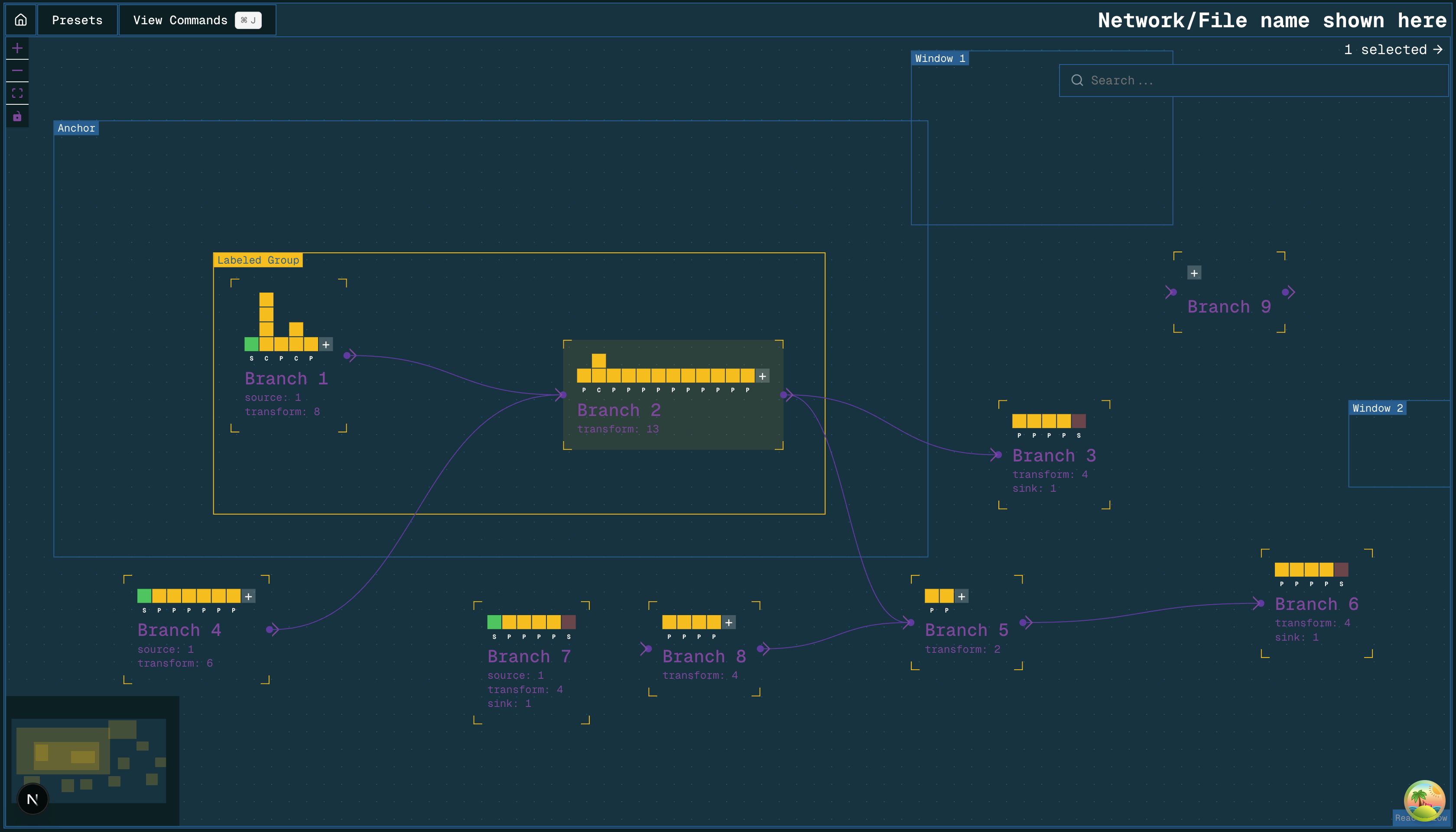 A directed graph representation of a flow network
Branches
A branch contains a linear sequence of blocks. It can be named. It has one inlet port and one outlet port, marked with an arrow head. Each port may be connected to any number of other branches. Connections are shown as lines between connected branches.
If a branch has multiple connections at its inlet port, it receives the combination of the inlet streams as its inlet fluid. If a branch has multiple connections at its outlet port, the split ratio can be determined by the user, with the default behaviour being an equal split. If a branch has either no inlet or no outlet connections, it must have the appropriate terminal block.
They are similar to blocks. They could even potentially be used to define compound blocks but that’s something to consider later.
There is no constraint on the number of blocks a branch may contain. A branch may be empty or contain one or many blocks. If you want to name a sequence of blocks (perhaps to represent an asset) you may create a branch containing those blocks.
Blocks
Blocks represent the components that exist within branches. They have their own properties. They correspond to components like pipes, compressors, heaters, and coolers (or sequences of multiple components). I am intentionally avoiding calling these components though.
Multiples of the same block may exist in parallel, and this is represented by vertically stacked blocks. When this happens, the incoming fluid flow is divided equally between the parallel blocks.
 An example branch with a block sequence of one source, four capture units, a pipe, two compressors, and another pipe
We can add to block sequences by extending them at the end or inserting blocks in the middle, much like you would add rows to an Excel data sheet, with the option to add a new block before or after a selected one. To add a block just before the two compressors, the user would click the blue area.
An example branch with a block sequence of one source, four capture units, a pipe, two compressors, and another pipe
We can add to block sequences by extending them at the end or inserting blocks in the middle, much like you would add rows to an Excel data sheet, with the option to add a new block before or after a selected one. To add a block just before the two compressors, the user would click the blue area.
Terminal blocks
A source block is where the composition and flow rate of a fluid stream are defined. This fluid is passed along to the next block in the sequence. A sink block is where a fluid stream terminates. One must be placed at the end of a branch if the branch is not connected to another.
Groups
Groups are a labeled container for branches. They can have their own properties which are accessible by the branches and blocks within. This is useful for defining conditions that apply to multiple branches but not all of them.
Map windows and anchors
We can display elements overlaid on a map by having placeable map elements on the user interface. An anchor is the one that sets the position and scale of the map. A window is a moveable island that provides a view of the same map in a different location.
Contexts and inherited values
We often say that we don’t want default values for any of our properties but this is only really true if you’re strictly talking about values the user had no say in or values that may quietly hide a misconfiguration. But some properties are defined globally or for groups of components. Some are determined by their position in the network. The user should not be made to manually enter every value for every property.
Consider mass flow: the total mass flow into Branch 2 in the above image is the sum of the flow from Branch 1 and Branch 4. The mass flow into Branch 3 and Branch 5 is determined by the mass flow and split ratio from Branch 2. A component within these destination branches may make use of the mass flow value, but you would not expect to need to enter it manually. Mass flow is clearly a branch-level property.
For some properties, it may be useful to define them at the group level. Ambient temperature is one example. Perhaps something like compressor efficiency too. In every case (barring fluid properties like mass flow, which is specifically branch-level only), I think it makes sense to allow properties to be defined in broader contexts and overridden by definitions in narrower contexts. Components should inherit the property values from the contexts they exist within.
This would allow the user to say “every pipe in this group has a U-value of X, but I will override this specific one with a U-value of Y” without any difficulty, by setting the group level property to be X and the value within a specific component to be Y.
Costing
For cost calculations, we define modules that contain cost items, each with their own properties, and group these into assets. As a cost item is the smallest unit, they should map onto blocks well. However we may also use a block to represent multiple cost items and should do so when they are indivisible.
If a pipe is always defined along with a road crossing, for example, we should use the block to represent both together. (This is true even if we might sometimes have a pipe with 0 road crossings as long as the road crossing can’t be defined independently of the pipe.)
It might be the case that one cost library says that every pipe should be represented as Item 001 but a later decision means that, going forward, new cost libraries will use Item 002 instead, or perhaps a combination of multiple cost items. For this reason, we should be able to describe the network without using the cost items themselves even if the goal is to map the elements onto cost items for evaluation.
Cost library
A cost library defines a set of cost items and their parameters.
We already group these into “modules,” which roughly correspond to what I call “blocks,” but there is open discussion about how these are grouped and represented. Both modules and blocks are sets of (one or many) cost items, but I’m using a new term to avoid inadvertently drawing from the existing concept. My idea of a block is something more stable than our existing modules, which may be redefined between different versions of a cost library.
A cost library should define the mapping between cost items and blocks. The goal would be to have a set of unchanging blocks to describe the network that you could assess with different cost libraries. We might say a network has a compressor block and a cost library would map that on to Item 013 or Item 015, depending on the version, or even present the user with a choice of multiple cost items. But I think it’s important that this is a separate layer.
Modelling
Describing the network as a directed graph of branches allows you to model each branch independently and see if they each produce the desired output. This is important when you have an incomplete network or you are working to meet constraints in multiple places. It allows you to ask the question “given that the fluid entering Branch 2 is X, what are the properties of the outlet fluid?” And that’s a question that our existing primary model is not designed for. Our primary model is a search function that answers the question “if one exists, what is a set of fluid properties that produce the right pressure at the reservoir?”
If you can do thermodynamic modelling of the fluid in each branch, you can use the calculated properties for costing too, for example where enthalpy change might be connected to a compressor’s duty.
Modelling calculations are used to inform cost calculations, but the specific cost item that is used for a pipe won’t change the frictional pressure loss calculation, for example, so this is another reason to consider the network as being made of blocks that map onto cost items rather than being made of cost items themselves: the fact that I’m using Item 001 isn’t particularly relevant for the thermodynamic calculations.
Thermodynamics
We can use tab files for thermodynamics but each one can only contain data for a single fluid composition. If we have multiple streams with different compositions, perhaps even mixing with varying flow rates, the number of required tab files would become large quickly if we want to faithfully represent all the thermodynamic data for every composition.
It has been mentioned that some impurities don’t produce significant differences in the thermodynamic data, so it might be possible to dramatically reduce the number of tab files used if we can ignore some of the differences in compositions and still get a reasonably accurate result.
Alternatively we would need a service to provide thermodynamic data. Tab files are a useful format because they are already a standard and we have a parser, so even if we don’t use Multiflash to produce these files directly it would be good if our service provided data in the tab file format.
Point evaluation
We can calculate the output of a set of components given a specific input fluid. This is exactly what you would expect for the forward pass calculations of the network elements. We pass an input to a function and get an output.
If the user has specific inputs they want to evaluate, these can be defined at the source blocks and passed downstream.
Parallelism
It is possible to process a whole range of inputs in parallel with WebGPU compute shaders. The thermodynamic data for a composition would be packed in to RGBA storage textures and component parameters would be passed as uniforms to the shaders.
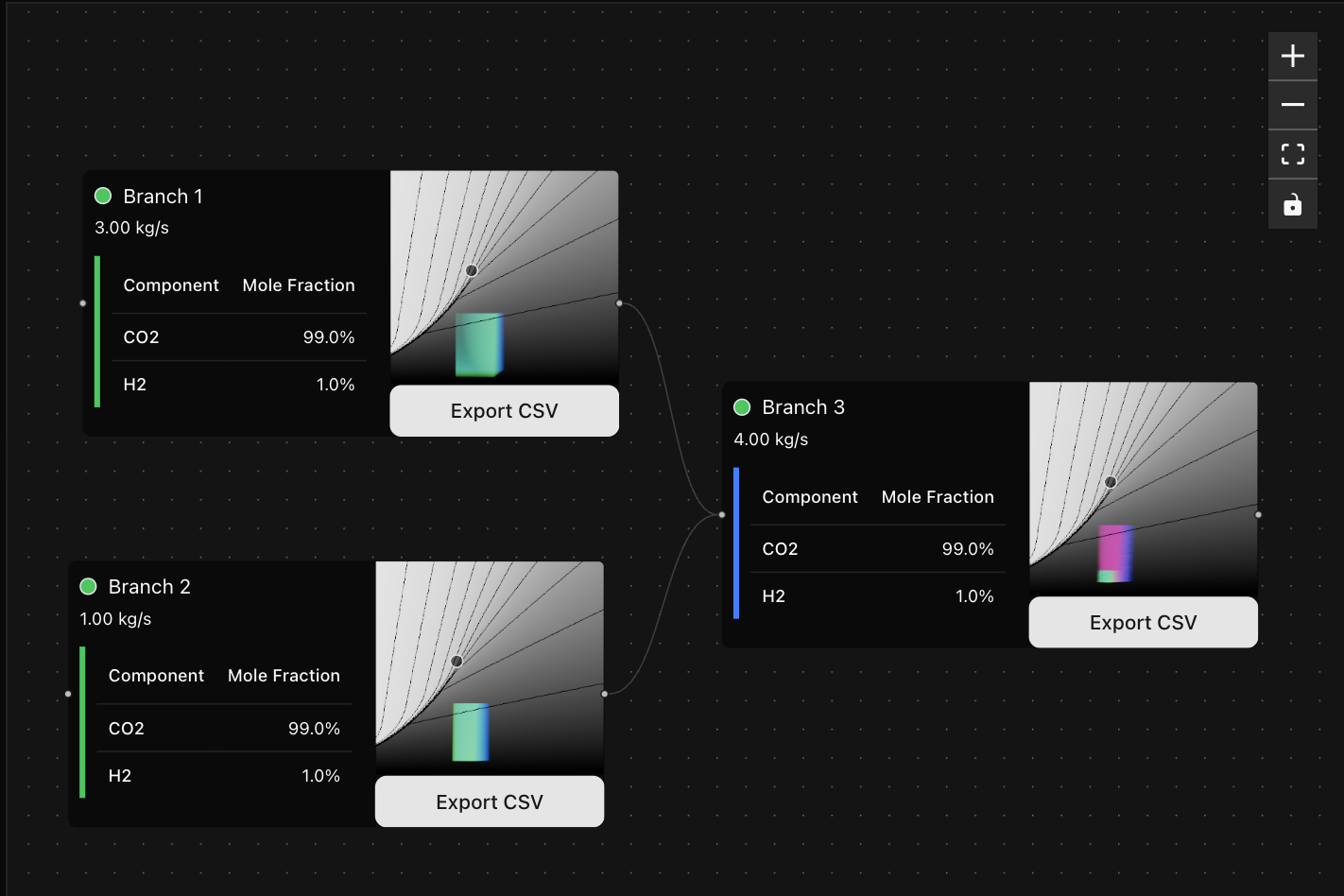 A shader-based approach to modelling inputs in parallel
The black/white gradients show enthalpy with isolines on a Pressure-Temperature axis. Thousands of blue-green lines show how input properties are mapped to another location in the phase diagram. Branch 3 applies a pressure constraint to the final position of the fluid trajectories, marking them as invalid with blue-red lines. Invalid candidate trajectories are culled and not passed on to the next branch.
A shader-based approach to modelling inputs in parallel
The black/white gradients show enthalpy with isolines on a Pressure-Temperature axis. Thousands of blue-green lines show how input properties are mapped to another location in the phase diagram. Branch 3 applies a pressure constraint to the final position of the fluid trajectories, marking them as invalid with blue-red lines. Invalid candidate trajectories are culled and not passed on to the next branch.
This approach tells you exactly where in your network a trajectory of fluid properties becomes invalid, clearly highlighting problem areas to the user. Every trajectory can be traced back to its original position.
These transformations and constraints on the input fluid properties can be completely arbitrary. It’s possible to define a reservoir that accepts fluid only within a certain pressure range, or have a compressor reject fluids that require a duty above a certain value (perhaps even setting the threshold based on cost).
This parallel modelling approach is similar to the genetic algorithm we used to evaluate different permutations of a network years ago. It involves creating and pruning a large number of candidate solutions. The goal is not to “draw your network on the phase diagram”. The phase diagram is just the space that can be used to define candidate solutions (See Modelling in increments), which you necessarily are doing every time you describe the properties of a fluid. The network would be built using an interface designed for that purpose, and can then be used to evaluate points in the phase diagram.
Every time we do a binary search to find a snapshot result, we are attempting to find a valid trajectory whether or not we describe it that way. We just also end up making the additional claim that this particular result is “the state of the network” when really it is just one of however many satisfy the constraints we set. We’re doing something that approximates this in a less rigorous and transparent way and presenting the outcome as something it isn’t.