Networks of fluid flow can be described as a series of connected branches.
A branch is a linear sequence of connected components through which the fluid flows. A branch may be connected at its ends to zero, one, or many branches.
Here is a diagram from an OLGA manual illustrating branches and nodes. This is similar to the way I independently modelled pipeline networks a couple years ago.
In this diagram, the internal nodes are hollow and the boundary nodes are filled in. The boundary nodes are the points where fluid enters or leaves the system - where you might define a combination of flow rate, composition, and pressure.
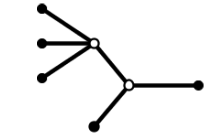
Going counter clockwise, I will call these boundary nodes A, B, C, D, and E.
User interface
As a user interface, this illustration method has some pitfalls, some with more obvious solutions than others.
If a the properties of a branch change meaningfully across its length (e.g. elevation profile), you need to introduce a concept of orientation to each one. In my model, I used a triangle to turn each branch into a kind of arrow.
If your calculation simply takes a set of fluid properties at the inlet of a pipe and passes it into a function that returns the outlet properties, and orientation is significant, you must know in advance which direction the fluid flows through the pipe. You could try to infer this by which end is connected to an inlet and which is connected to an outlet, but this becomes more difficult when you move past the simplest network shapes.
You might have imagined the illustration above as a network with four inlet points and only a single outlet point at the rightmost boundary node, but this is not the only possible configuration. The alignment of the boundary nodes A, B and C suggets that the fluid flows from the left, merging into a single branch, and continues rightwards. But that it not necessarily true.
If it is possible for the user to define any combination of boundary nodes as inlet and outlet points, you no longer know the flow direction in each branch. If boundary nodes A, C, and D were outlets and all the rest inlets, it becomes much less clear which way we expect fluid to flow.
If instead of defining flow rates at each boundary node, they defined pressures, flow direction would be determined by the pressure differences between the ends of each branch.
It is possible to form a network with loops. Or to use angles that make the intended flow direction less obvious. You could say that you won’t model networks with loops. Fine.
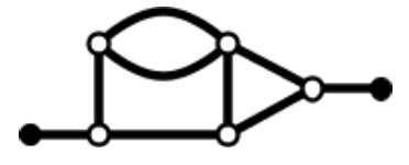
But after using this method to draw networks, it becomes clear that asymmetrical branches need something more. Using lines to draw pipes might sound good at first but if a pipe is not symmetrical across its length then it shouldn’t be visually represented as a uniform line. Things become clearer when you define a side for the fluid to enter or leave the branch. It is better instead to fix the orientation of the branches.
The “fixed orientation” approach could look something like this, where each branch is represented by a box and the orange lines between them are “logical” connections rather than physical pipes. It’s a graph where the branches are nodes and the links represent the connections between branches.
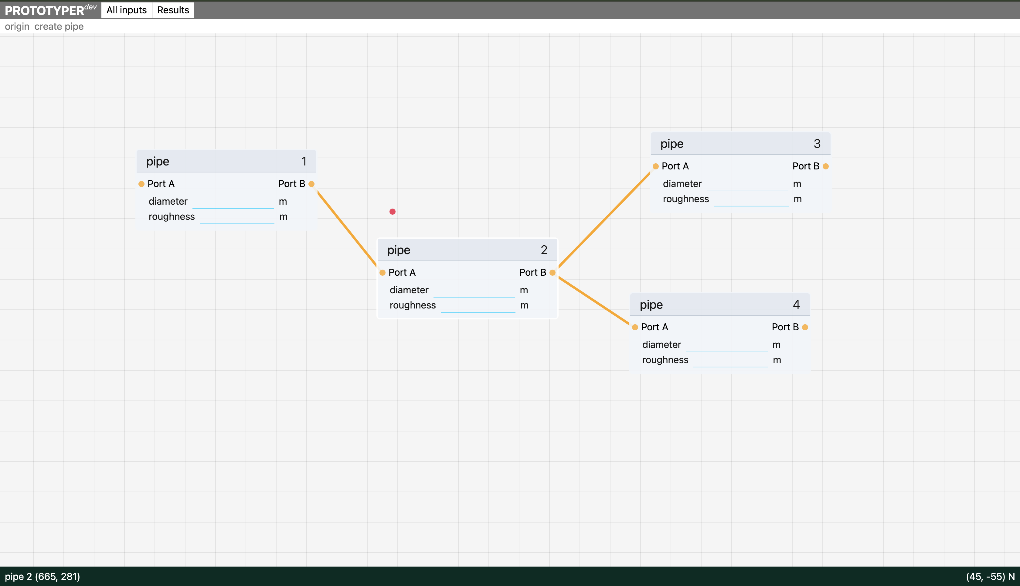
The property fields (diameter, roughness) in each box are more illustrative than necessary. Each branch would have its own set of properties that may or may not vary across its length. If you really wanted to rotate these, that could be possible, but the important thing is to know whether you’re connecting to Port A or Port B. Because the elevation at ports A and B may differ. The expectation though is that things flow from left to right, Port A to Port B.
Here is a more refined version of the concept, where a branch may be composed of multiple components, rather than just being a length of pipe.
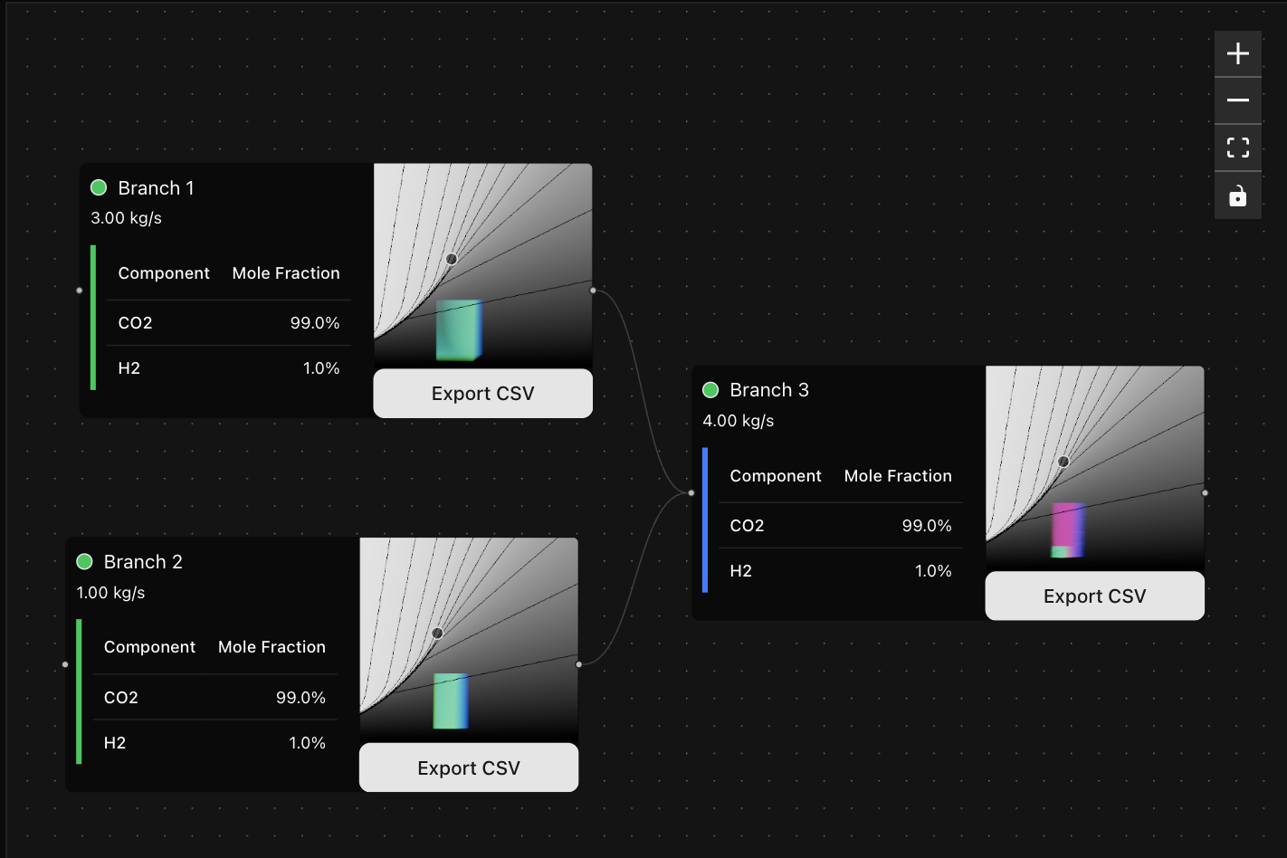
In this version of the network model, a branch contains an ordered list of components. I have called the nodes on the left and right of each branch ports. If a branch has nothing connected to its inlet port, it must have a defined set of Source properties: a pressure range, a temperature range, and a flow rate. Where a branch has upstream branches connected to its inlet port, its incoming fluid is calculated by combining the fluid from each of its sources.
The phase diagrams on each branch show the trajectories of all fluids within the source property range at the specified flow rate.
Each component in the branch applies a transformation or constraint to the incoming fluid. A transformation takes fluid properties at one position on the phase diagram and calculates where that fluid is moved to. A constraint determines whether the incoming fluid properties are acceptable, marking unacceptable properties as invalid trajectories. The trajectories are shown as blue-green lines for valid trajectories and blue-red lines for invalid trajectories.
Reservoirs are examples of components that may mark a fluid trajectory as invalid. In the above network, branch 3 uses a Reservoir component to mark as invalid any trajectory that ends above the allowed pressure limit.
Assets
It is useful to be able to group a series of connected components as an asset that may be named or moved to another location, or swapped with another asset for comparison.
In my network model, those are easily represented as branches. There is no requirement to have branches of a certain size, so you could easily have a “branch” that represents an asset within one larger leg of the network.
Grids
There is a temptation to place these elements on a grid but it should be considered whether grid position is a meaningful part of the data model. One iteration produced at work involved a grid where each row was a branch, each branch starts from the left of the grid, and everything flowed from left to right.
If you stop to consider the shapes a network might have, it becomes clear that this is not flexible enough: two merging branches may not have the same length. The merging branches may not occupy neighbouring rows in the grid. Now you have to draw lines to distant cells and you start questioning why things are on the grid to begin with.
You don’t even get to entertain the idea of a network that splits because that means modules in the same row are not necessarily part of the same branch.
These things should be an indication that this is not a good way to represent flow networks.
Directed graph
The most natural way to represent these networks is as a directed graph of branches where each branch has an ordered list of components.
Each branch is a node in the directed graph and the links just represent connections. And it is still possible to align these nodes on a grid, but that would be a choice. You could quite easily imagine each branch (or even each module within a branch) in the images above filling a grid cell.